We recently reduced CPU usage across our fleet by 80%. One key technique that made this possible was a lightweight profiling strategy that we could run in production. This post is about the ways we approached instrumentation, the tradeoffs involved, and some tools you can use to optimize your own apps (including code!).
Background
Nylas is a developer platform that provides APIs to integrate with email, contacts, and calendar. At the core of this is a technology we call the Sync Engine. It’s a large Python application (~30k LOC) which handles syncing via IMAP, SMTP, ActiveSync, and other protocols. The code is open source on GitHub with a solid community.
We run this as managed infrastructure for developers and companies around the world. Their products depend on our uptime and responsiveness, so performance of the system is a huge priority.
If You Can’t Measure It, You Can’t Manage It
Optimization starts with measurement and instrumentation, but there’s more than one way to profile. It’s important to be able to profile both at small scale using test benchmarks, and at large scale in a live environment.
For example, when a new mailbox is added to the Nylas platform, it’s essential that messages are synced as quickly as possible. To optimize this, we need to understand how different sync strategies and optimizations affect the first few seconds of a sync.
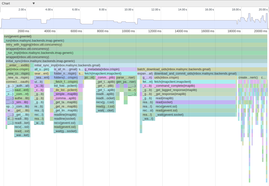
By setting up a local test and adding a bit of custom instrumentation, we can build up a call graph of the program. This is simply a matter of using sys.setprofile() to intercept function calls. To better see exactly what’s happening, we can export this call graph to a specific JSON format, and then load this into the powerful visualizer built into the Chrome Developer Tools. This lets us inspect the precise timeline of execution:
Doing it live
This strategy works well for detailed benchmarking of specific parts of an application, but is poorly suited to analyzing the aggregate performance of a large-scale system. Function call instrumentation introduces significant slowdown and generates a huge amount of data, so we can’t just directly run this profiler in production.
However, it’s difficult to accurately recreate production slowness in artificial benchmarks. The sync engine’s workload is heterogeneous: we sync accounts that are large and small, with different levels of activity, using different strategies depending on mail provider. If the tests aren’t actually representative of real-world workload, we’ll end up with ineffective optimizations.
Our answer to these shortcomings was to add lightweight instrumentation that we could continuously run in our full production cluster, and design a system to roll up the resulting data into a manageable format and size.
At the heart of this strategy is a simple statistical profiler – code that periodically samples the application call stack, and records what it’s doing. This approach loses some granularity and is non-deterministic. But its overhead is low and controllable (just choose the sampling interval). Coarse sampling is fine, because we’re trying to identify the biggest areas of slowness.
A number of libraries implement variants of this, but in Python, we can write a stack sampler in less than 20 lines:
import collections
import signal

class Sampler(object):
  def __init__(self, interval=0.001):
    self.stack_counts = collections.defaultdict(int)
    self.interval = 0.001

  def _sample(self, signum, frame):
    stack = []
    while frame is not None:
      formatted_frame = '{}({})'.format(
        frame.f_code.co_name,
        frame.f_globals.get('__name__'))
      stack.append(formatted_frame)
      frame = frame.f_back
    formatted_stack = ';'.join(reversed(stack))
    self.stack_counts[formatted_stack] += 1
    signal.setitimer(signal.ITIMER_VIRTUAL, self.interval, 0)

  def start(self):
    signal.signal(signal.VTALRM, self._sample)
    signal.setitimer(signal.ITIMER_VIRTUAL, self.interval, 0)
Calling Sampler.start() sets the Unix signal ITIMER_VIRTUAL to be sent after the number of seconds specified by interval. This essentially creates a repeating alarm that will run the _sample method.
When the signal fires, this function saves the application’s stack, and keeps track of how many times we’ve sampled that same stack. Frequently sampled stacks correspond to code paths where the application is spending a lot of time.
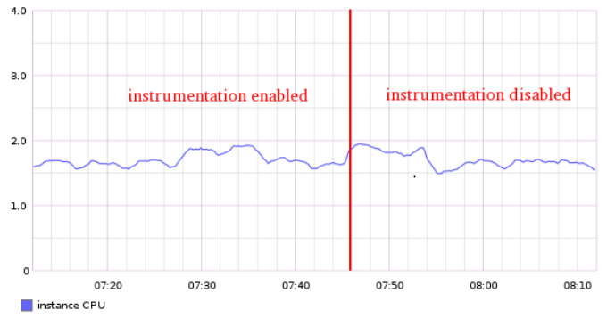
The memory overhead associated with maintaining these stack counts stays reasonable, since the application only executes so many different frames. It’s also possible to bound the memory usage, if necessary, by periodically pruning infrequent stacks. In our application, the actual CPU overhead is demonstrably negligible:
Now that we’ve added instrumentation in the application, we have each worker process expose its profiling data via a simple HTTP interface (see code). This lets us take a production worker process and generate a flamegraph that concisely illustrates where the worker is spending time:
curl $host:$port | flamegraph.pl > profile.svg
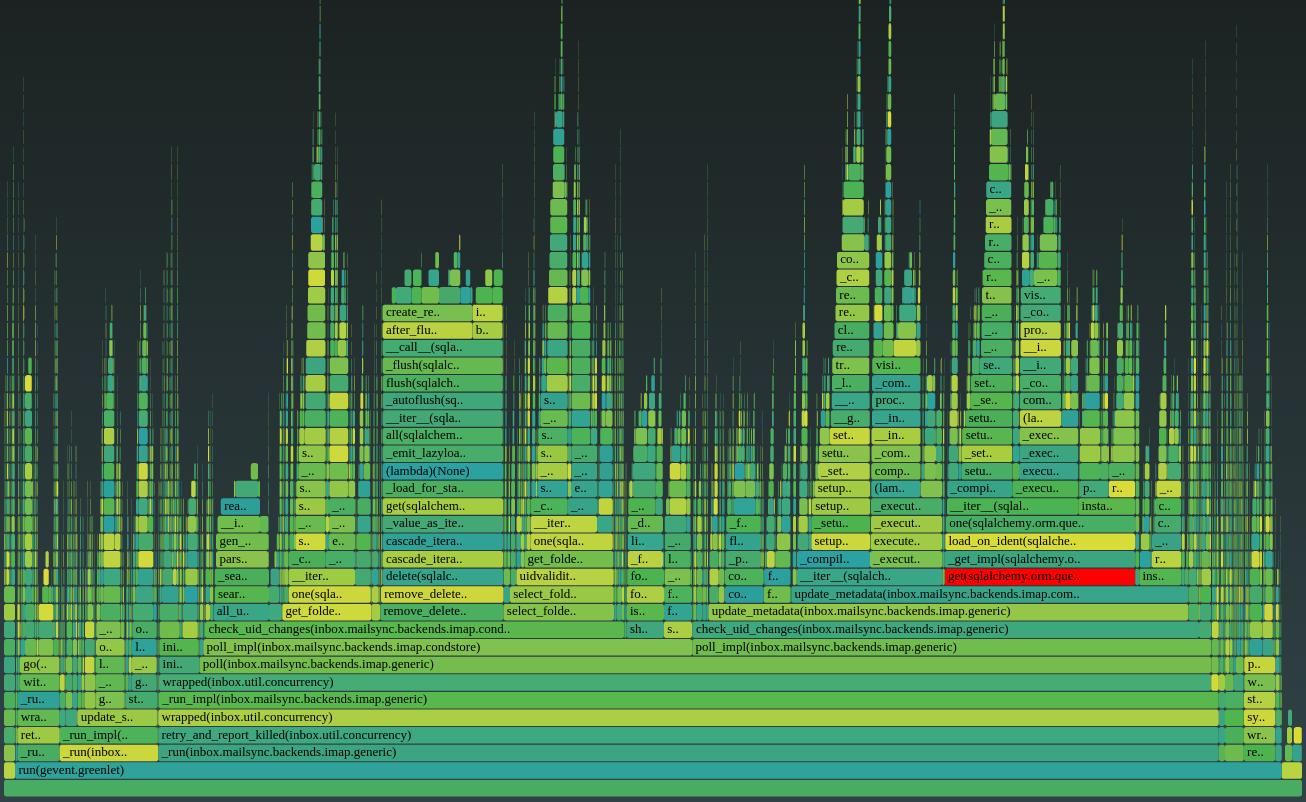
This visualization makes it easy to quickly spot where CPU time is being spent in the actual process. For example, around 15% of runtime is being spent in the get() method highlighted above, executing a database load that turns out to normally be unnecessary. This wasn’t evident in local testing, but now it’s easy to identify and fix.
However, the load on any single worker process isn’t necessarily representative of the aggregate workload across all processes and instances. We want to be able to aggregate stacktraces from multiple processes. We also need a way to save historical data, as the profiler only stores traces for the current lifetime of the process.
To do this, we run a collector agent that periodically polls all sync engine processes (across multiple machines), and persists the aggregated profiling data to its own local store. Because we’re vending data over HTTP, this is really straightforward; there’s no need to tail and rotate any files on production instances.
Finally, a lightweight web app can visualize this data on demand. Answering the question, “Where is our application spending CPU time?” is now as simple as visiting an internal URL:
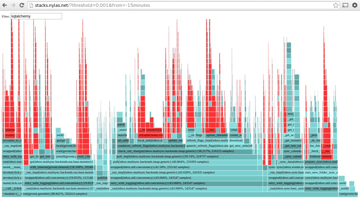
Because we can render profiles for any given time interval, it’s easy to track down the cause of any regressions and the moment they were introduced.
The code for all this is open source on GitHub– take a look and try it yourself!
Results
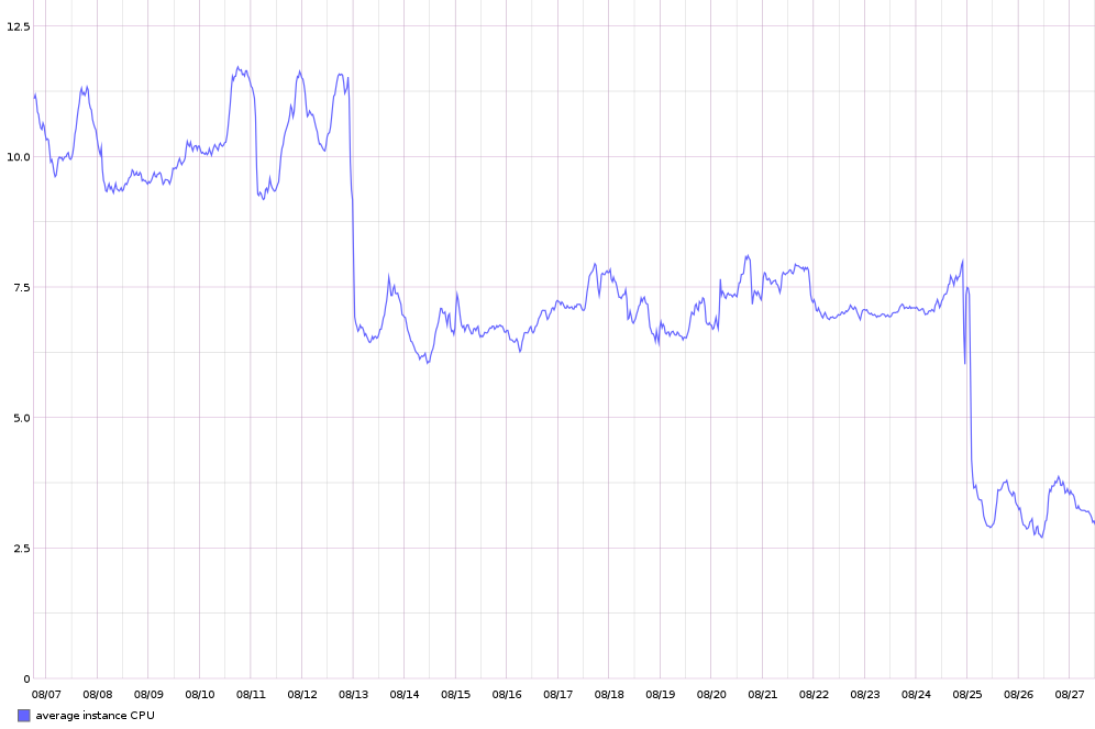
Having deployed this instrumentation, it was easy to identify slow parts of our managed sync engine and apply a variety of optimizations to speed things up. The net result was an 80% reduction in CPU load. The graph shows the effects after two successive sets of optimization patches were shipped.
Being able to measure and introspect our services in a variety of ways is crucial to keeping them stable and performant. The simple tooling presented here is just one part of the larger monitoring infrastructure at Nylas. We hope to cover more of that in future posts.
Related article:
Paying back technical debt: Lessons learned from scaling infrastructure by 20x
 Email and Contacts API
  Calendar API & Scheduler
  Notetaker API
  Agent Accounts


